Path Distance: adding more cost complexity |
|
|
Release 9.3
Last modified January 13, 2012 |


|
Note:
This topic was updated for 9.3.1.
The Path Distance functions are one group of several ArcGIS Spatial Analyst tools used for distance analysis. In conjunction with the Cost, Euclidean, Hydrologic, and other ArcGIS Spatial Analyst functions, many dispersion and movement processes can be effectively modeled. The next sections describe the basic theory behind the Path Distance function and how to use it.
Learn how to calculate path distance using the Path Distance tool
The basic rules of motion behind Path Distance
The Path Distance function is similar to the Cost Distance function in that both determine the minimum accumulative travel cost from a source to each cell location on a raster. However, Path Distance not only calculates the accumulative cost over a cost surface, it does so while compensating for the actual surface distance that must be traveled and for the horizontal and vertical factors influencing the total cost of moving from one location to another. The accumulated cost surface produced by the Path Distance function can be used in dispersion modeling, flow movement, and least-cost path analysis.
To make the most efficient use of Path Distance, you must understand some basic principles of dispersion and movement over a surface. To illustrate these basic principles, the amount of energy will be explored, or more explicitly, the amount of fuel needed to drive a car between two points while encountering various cost factors.
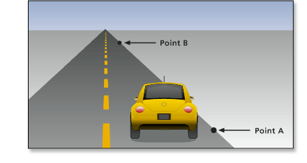
To drive a car on a flat road 50 miles from point A to point B will require x gallons of fuel.
More fuel will be needed to drive the same car from point A to point B if it has to travel on a rough or bumpy surface, such as an unpaved road. The amount of fuel used in the second instance is calculated by the distance traveled over the friction, which is the friction factor (F), to compensate for the bumpiness of the surface, times the distance to travel divided by the miles per gallon the car gets on flat, smooth surfaces (D = Miles traveled / miles per gallon), resulting in the following formula:
F * D = fuel used
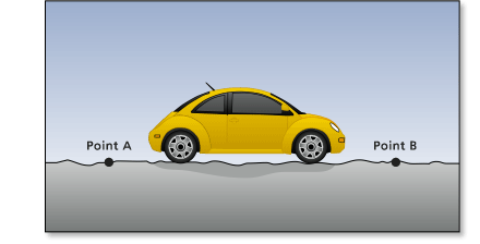
The above formula can also be used in the first example, but the friction factor was much lower than in the second example because the car traveled on a smooth surface.
If the route from point A to point B was uphill, the car would have to travel farther in actual distance than if the route were flat. (You can ignore for the moment the fact that additional fuel would be necessary to propel the car uphill.) The distance that would be traveled is referred to as the surface distance (SD).
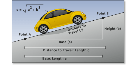
The surface distance extends the actual travel distance over the type of travel surface. Continuing the preceding example, the car now must travel on the bumpy surface for a longer distance. The surface distance (SD) increases the total cost of travel as a factor, not by simple addition. When considering surface distance (SD replaces D), the following formula is used:
F * SD = fuel used
Another group of elements that might influence a car's consumption of energy is the horizontal factors. These factors consider the easiest horizontal route to travel and how far from it the car is traveling. One horizontal factor in this example could be wind speed. If there is a strong wind behind the car it will use less fuel to move from point A to B, regardless of the surface and actual travel distance.
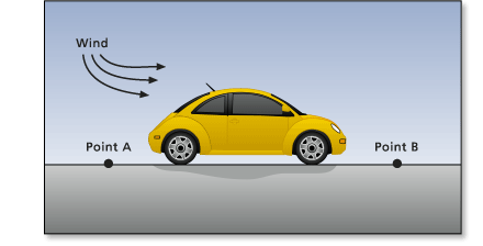
Including the horizontal factor (HF) in the total cost of travel results in the following formula:
F * SD * HF = fuel used
The horizontal factor related to wind speed must be adjusted to compensate for the amount of horizontal friction that will be encountered with regard to the relationship of direction of travel and wind direction. For example, if the wind is blowing behind the car at a 45-degree angle offset, the wind will be of some advantage to the car but not as much as if blowing directly behind it (a zero degree offset).
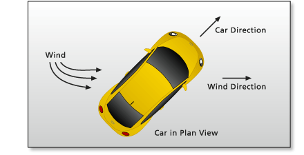
If the car is heading directly into the wind, the horizontal friction factor would be greatest.
The final factor that will affect the energy consumption of the car is the uphill or downhill slope that must be overcome during travel, which is called the vertical factor. In this example, if the car is going downhill, the total cost of travel will decrease; if it is going uphill, the total cost will increase.
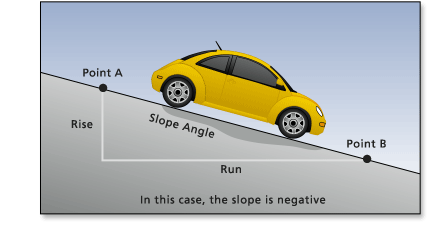
Incorporating the vertical factor (VF) into the previous formula results in the following formula:
F * SD * HF * VF = fuel used
When modeling a source of dispersion or a moving object, the Path Distance function will allow for control of the friction, surface distance, horizontal factor, and vertical factor. The example presented above is a simple one, but many of the elements affecting motion can be illustrated. Most movement is not as simple as a car traveling on a surface. For instance, it may be least costly for some types of phenomena when the vertical angle is great or when it deviates significantly from the specified horizontal direction of travel. Zero slope may be costly to overcome in another situation. Slope for the vertical factors may be air densities, concentration levels, or noise decibels rather than elevation. The Path Distance function allows for the control of the factors that influence dispersion, such as the ones listed here, allowing for customization of the analysis to meet the requirements of the phenomena under consideration.
The theory behind Path Distance
How Path Distance calculates cost
The processing that occurs in Path Distance is similar to that of Cost Distance (see Understanding cost distance analysis). First the source cells are identified. Then the cost to travel to each neighbor that adjoins a source cell is determined. Next, each of the neighbor cells is listed from least costly to most costly. The cell location with the least cost is removed from the list. Finally, the least accumulative cost to each of the neighbors of the cell that was removed from the list is determined.
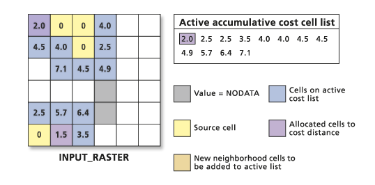
The process is repeated until all cells on the raster have been assigned an accumulative cost. The difference between the Cost Distance and Path Distance functions is how the cost of moving from one cell to the next is computed (see Cost Distance algorithm). This section examines each of the input rasters and parameters as well as the formula used to calculate total accumulative cost for Path Distance. The parameters for Path Distance are:
- Source raster
- Cost (distance) raster
- Surface raster
- Horizontal factor raster
- Horizontal factor parameter
- Vertical factor raster
- Vertical factor parameter
- Output back link raster
- Maximum distance
The first seven parameters for Path Distance are the inputs necessary for determining the cost to travel between any two adjacent cells. The last two arguments affect the output and its format.
The formula used to calculate the cost of travel from cell a to cell b (where b is one of a's eight directly connected neighbors) is:
Cost_distance = Cost_Surface * Surface_distance * {[Friction(a) * Horizontal_factor(a) + Friction(b) * Horizontal_factor(b)]/2} * Vertical_factor
The additional distance necessary to travel diagonally is compensated when calculating the surface distance component (1.414214 * distance) of the above formula.
The accumulative cost to travel from cell a to cell c passing through cell b is:
Accum_cost_ distance = a1 + Surface_distance * Vertical_factor * {[Friction(b) * Horizontal_factor(b) + Friction(c) * Horizontal_factor(c)]/2}
where:
a1 is the total cost of travel from cell a to cell b
The source raster
The source raster identifies those cells from which a least accumulative cost distance is calculated to each nonsource cell. The source raster for Path Distance is identical to the source raster for Cost Distance.
The cost raster
The cost raster is identical to the cost raster in the Cost Distance function. Each cell location is given a weight proportional to a relative cost incurred by the phenomena being modeled when passing through a cell. The costs are usually based on inherent features in the location that are static prior to the movement of the feature or phenomena. If modeling fire movement, for example, the cost features might include slope, aspect, age, type, moisture content, and canopy cover of the vegetation.
The cost units are based on any relative scale. The units can be dollar cost, energy units expended, or preference costs can be unitless. What is most important is that the values be in a relative scale. Adding the values associated with slope, aspect, and vegetation type will give meaningless results to fire movement. However, if each of these attributes is reclassed in relation to fire susceptibility, then added, the results will be a fire cost raster.
The cost values assigned to each cell are per unit distance measures for the cell. That is, if the cell size is expressed in meters, the cost assigned to the cell is the cost necessary to travel one meter within the cell. If the resolution is 50 meters, the total cost to travel either horizontally or vertically through the cell would be the cost assigned to the cell times the resolution (total cost = cost * 50). To travel diagonally through the cell, the total cost would be 1.414214 times the cost of the cell times the cell resolution [total diagonal cost = 1.414214 (cost * 50)].
By interpreting the costs stored at each cell as the cost-per-unit distance of travel through the cell, the analysis becomes resolution independent. Suppose there are two rasters, one at 50-meter resolution and the other at 100-meter resolution. Several adjoining cells in each raster are assigned five cost units to travel through each cell. The five cost units are applied to each unit of distance (the cost to move a meter in this case); therefore, it will cost 500 cost units to move 100 meters through the cells in either of the two rasters regardless of their resolution.
The Path Distance function creates an output raster in which each cell is assigned the accumulative cost from the cheapest source cell. The algorithm utilizes the node/link cell representation. In this representation, the center of a cell is considered a node, and each node is connected by links to the nodes adjacent to it.
Every link has an impedance associated with it. The impedance is derived from the costs associated with the cells at each end of the link (from the cost surface) and from the direction of movement. In moving from a cell to one of its four directly connected neighbors, the cost to move across the links to the neighboring node is the cost of cell 1 plus the cost of cell 2, divided by 2:
    a1 = (cost1 + cost2) / 2

    where:
      cost1 is the cost to travel through cell 1
      cost2 is the cost to travel through cell 2
      a1 is the cost assigned to the link from cell 1 to cell 2
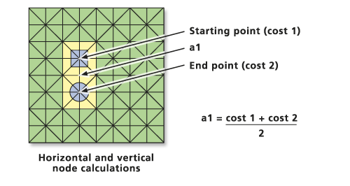
The accumulative cost is determined with the following formula:
    accum_cost = a1 + (cost2 + cost3) / 2

    where:
      cost2 is the cost to travel through cell 2
      cost3 is the cost to travel through cell 3
      accum_cost is the accumulative cost of moving into cell 3 from cell 1
      (note: a2 in the image below is the cost of moving from cell 2 to cell 3)
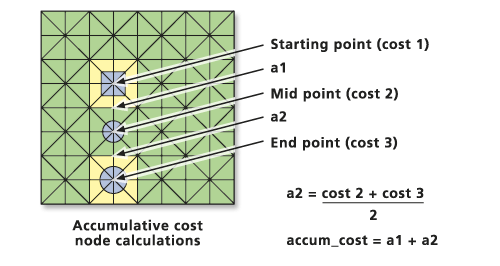
If the movement is diagonal, the cost to travel the link is 1.414214 (the square root of two) times the cost to travel through cell 1 plus the cost to travel through cell 2, divided by two:
a1 = 1.414214(cost1 + cost2) / 2
When determining the accumulative cost for diagonal movement, the following formula is used:
accum_cost = a1 +1.414214(cost2 + cost3) / 2
The cost surface (cost friction) accounts for the first element in the Path Distance formula:
Cost_distance = Cost_Surface * Surface_distance * {[Friction(a) * Horizontal_factor(a) + Friction(b) * Horizontal_factor(b)]/2} * Vertical_factor
The division of the friction of the segments by two is deferred until the horizontal factor is integrated.
The surface raster
The surface raster is used to determine the actual surface distance traveled from one cell to the next. Elevation is usually the input surface raster. The Pythagorean theorem is used to calculate the actual travel distance from cell a to cell b:
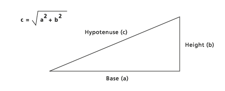
If the cost is calculated to one of the four adjacent neighbors, the length of the base (a) is equal to the cell size (the distance from the center of one cell to the center of another). If the cost is determined to a diagonal cell, the base is derived from the cell size times 1.414214. To determine the height (b) of the triangle, the height of the To cell on the surface raster is subtracted from the height of the From cell.
When the surface is not flat, the travel distance is greater. Greater distance means that more cost is incurred at the rate determined by the input cost raster and by the horizontal and vertical factors.
The surface raster is used to determine the actual surface distance traveled from one cell to the next. The cost of overcoming the angle of incline or decline (slope) is not necessarily calculated from the surface raster. The costs associated with the slope angle are calculated from the input vertical factor raster and accompanying vertical cost factors. The raster used for the vertical factor raster can be the same as the raster used for the input surface raster.
The surface distance accounts for the second element in the Path Distance formula:
Cost_distance = Cost_Surface * Surface_distance * {[Friction(a) * Horizontal_factor(a) + Friction(b) * Horizontal_factor(b)]/2} * Vertical_factor
The horizontal factors
The horizontal factor influences the total cost of moving into a cell by accounting for any horizontal friction encountered. To calculate the total HF for traveling between cells, the HF for the segment of the link from the center of the processing cell to the edge of the To cell and for the segment of the link from the edge of the To cell to its center must be determined.
Determining the horizontal cost for each link is a two step process. First, the prevailing horizontal direction must be established. A horizontal direction is defined in degrees, with zero being above, or north, of the processing cell and the values increasing clockwise, creating a circle and returning onto itself at 360 degrees.

The horizontal direction is defined by a value assigned to each cell location on the input horizontal-factor raster.
The horizontal direction defined for each cell often identifies the direction with the lowest horizontal cost of movement with respect to the processing cell. This does not necessarily have to be the case.
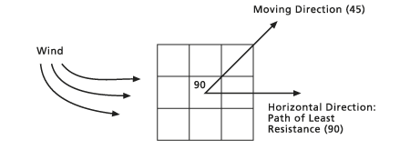
Once the horizontal direction has been defined, the horizontal factor used in calculating the total cost of moving along the segment must be determined. First, the position of the To cell relative to the horizontal direction must be ascertained. The direction of the To cell relative to the prevailing horizontal direction at the From cell is the horizontal moving direction or just the moving direction. The number of degrees or angle of the To cell from the horizontal direction as defined by the horizontal-factor raster is the horizontal relative moving angle (HRMA).
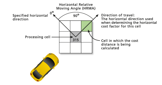
The number of degrees from the established horizontal direction, not which side of the established direction, is of relevance.
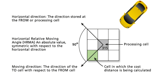
Once the HRMA has been determined, a graph is used to identify the actual horizontal factor. The HF is on the y-axis, and the HRMA is on the x-axis.
In the example above, if the cell whose horizontal factor you are calculating has an HRMA of 90 degrees from the horizontal direction as defined by the processing cell on the input horizontal factor raster, the horizontal-factor cost will be 1.61.
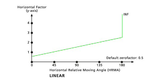
The HRMA values can range from -180 to 180 degrees. However, on the horizontal factor graph, the values on the x-axis are from 0 to 180 because the graph is assumed to be symmetrical (mirrored) around the horizontal factor axis; that is, 180 degrees is opposite the direction specified by the horizontal direction raster, and 90 degrees is to the right and left of the processing cell. INF means the line goes to infinity.
This same process is performed for the segment starting at the edge of the To cell and ending at its center. The moving direction remains the same, but the horizontal direction that will be used for the calculations is the prevailing horizontal direction at the To cell. Dividing the travel link between two cells into two segments (half the segment being in the From cell and the other half in the To cell) will give a more accurate horizontal factor since half the distance from the From cell to the To cell encounters the cost associated with the From cell; the remainder of the distance will be in the adjoining cell, which has a different horizontal resistance. In the Path Distance formula, each segment's horizontal factor is multiplied by its respective cost factors determined from the cost raster.
The horizontal cost factor accounts for the third element in the Path Distance formula:
Cost_distance = Cost_Surface * Surface_distance * {[Friction(a) * Horizontal_factor(a) + Friction(b) * Horizontal_factor(b)]/2} * Vertical_factor
The horizontal factor graph
The horizontal factor graph that will be used to determine the horizontal factor can be defined by either choosing an existing graph from the graphs provided with the software or creating a custom graph from an ASCII file. The existing graphs provided with the software are the following:
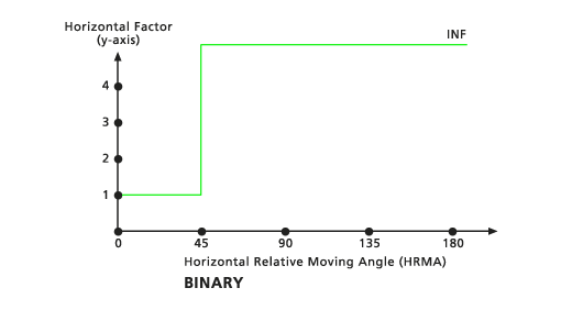
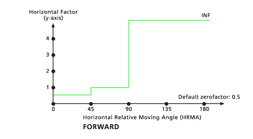

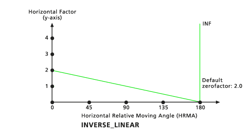
To create a graph from an ASCII file, any text editor can be used. The file consists of two columns. The first contains the HRMA, which is expressed in degrees, and the second, the HF. Each line in the file specifies a point on the graph. Two consecutive points define a line segment in the HRMA-HF coordinate system. The HRMA angles must be entered in ascending order.
The following is a sample horizontal factor ASCII table:
0 1.40
10 2.43
20 2.30
30 3.44
40 1.25
50 1.02
60 0.90
70 0.86
80 0.25
90 0.78
100 1.49
110 2.35
120 3.32
130 2.39
140 3.18
150 2.13
160 1.89
170 1.20
180 2.034
Several of the HRMA keyword parameters have modifiers that can be specified to achieve various desired results. The slope of the line in the LINEAR and INVERSE_LINEAR functions, the side values for the FORWARD function, and the zero factor can alter the y-axis intercept for the input functions, and the cut angle for any of the HRMA functions can all be controlled. Do not be concerned if you are unfamiliar with the effects of the modifiers at this point. Just be aware that you are able to further control the HRMA graphs to meet your needs.
The vertical factor
The vertical factor takes into account the cost necessary to overcome the slope between two cells. Determining the vertical factor encountered when traveling from one cell to another is similar to determining the horizontal factor. The vertical slope or angle is first calculated between cells from the z-values assigned to each location on an input vertical factor raster; the slope is then correlated to a vertical factor on a graph.
However, the link traveled in determining the VF is not broken into two segments as when calculating the HF. This is because there is only one slope between the two cell centers; hence, there is only one vertical relative moving angle (VRMA).
To determine the vertical slope or angle between two cells, the vertical values for each location must be identified from the input vertical-factor raster. The slope is calculated using the Pythagorean theorem. The base of the triangle necessary for determining the slope is derived from the cell size. The height is established by subtracting the From cell value from the To cell value. The resultant angle is the VRMA.
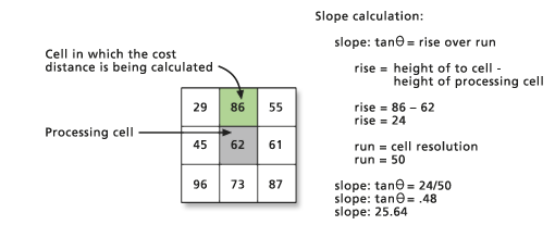
Once the VRMA has been determined, the specified graph is consulted. The vertical factor is on the y-axis of the graph, and the VRMA is on the x-axis. The VRMA, which can range from -90 to 90, is matched on the graph and a VF is determined.
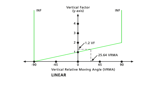
The vertical factors account for the fourth and final element in the Path Distance formula:
Cost_distance = Cost_Surface * Surface_distance * {[Friction(a) * Horizontal_factor(a) + Friction(b) * Horizontal_factor(b)]/2} * Vertical_factor
The vertical factor graph
Defining the vertical factor graph that will be used when determining the VF involves the same steps as defining the horizontal factor graph. The graph can be selected from a list of graphs provided with the software, or you can create a custom graph with an ASCII file. The vertical factor graphs provided with ArcGIS Spatial Analyst include the following:
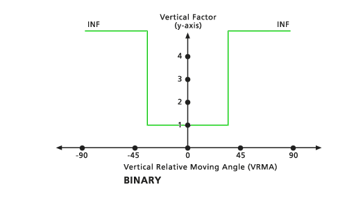

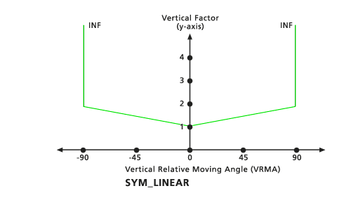
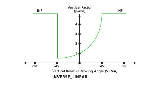
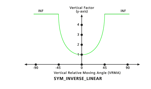
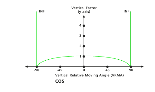
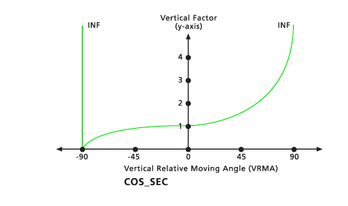
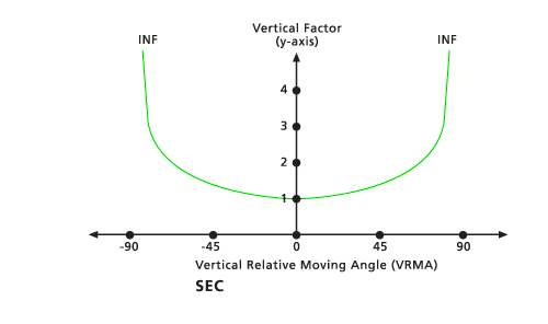
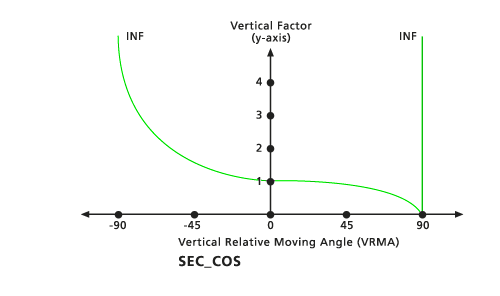
Creating a vertical factor graph from an ASCII file is similar to creating a horizontal factor graph. The file consists of two columns: one for the VRMA and a second for the VF. Each line in the ASCII file defines a point on the graph, and consecutive points create line segments in the VRMA-VF coordinate system.
As with an HRMA graph, the character of the VRMA graph can be further controlled by modifiers that allow for refinement of the vertical factors. The cut angles, which are discussed in the next section, can be specified for each of the functions, the trigonometric curves can be raised by a power, the zero factor can alter the y-axis intercept for the nontrigonometric functions, and the slope of the line in the linear functions can be defined. For more information on the VRMA modifiers, refer to the Path Distance command reference.
Cut angles
There may be a threshold angle such that if the HRMA or VRMA exceeds this angle, the cost is so great that it becomes a barrier to travel. This threshold is referred to as the cut angle. The HF or VF is assigned to infinity when the HRMA or VRMA exceeds the cut angle.
The horizontal factor graph will have a single cut angle, while the vertical factor graph will have both lower and upper cut angles.
Output rasters
In Map Algebra, three output rasters can result from Path Distance, one of which is mandatory. The mandatory raster is the output total accumulative cost distance raster. This raster stores the least cost accumulated distance for each cell that results from the least costly source cell. The accumulative cost distance raster is named to the left of the input expression for Path Distance in Map Algebra. An example expression is:
out_dis = pathdistance(source, friction, elev, in_hor, linear, in_vert, cos, out_back, out_alloc)
The two optional output rasters are the back link raster and the allocation raster. They are identified as input parameters in the above expression, with out_back standing for the output back link raster and out_alloc for the output allocation raster. The back link and allocation rasters are the same as those that result from the Cost Distance function.
The back link raster contains values from 0 through 8, which are codes that identify the direction to the next neighboring cell (the subsequent cell) when retracing (from the destination to the least costly source) the least accumulative cost path. If the path passes into the neighbor to the right, the cell will be assigned the value 1, 2 will be assigned for the lower-right diagonal cell, continuing clockwise. The value 0 is reserved for source cells.
The cost allocation raster identifies for each cell the zone of the source cell that can reach the cell location while accumulating the least cost.
In the geoprocessing environment, the three output rasters are derived from three separate functions: Path Distance (which can optionally create the back link raster), Path Distance Back Link (which can optionally create the distance raster), and Path Distance Allocation (which can optionally create the distance and the back link rasters).
Defining a maximum distance threshold
Sometimes a threshold accumulative cost is reached beyond which you are interested. Such a threshold is controlled by the maximum distance parameter. Any location that exceeds the threshold will receive NoData on the output cost distance raster.
Using alternative values on the allocation output raster
If the values associated with the source cells on the input source raster are to be replaced by alternative values on the output allocation raster, a value raster can be input. The values defined for each source cell by the value raster will be assigned to all cells that are allocated to the source cell location in the cost allocation raster.
Variations on the elements
Many variations can be modeled with Path Distance by altering one or all input parameters. For instance, if there is no input surface raster to calculate surface distance, nor horizontal or vertical factor cost elements, Path Distance will perform the same calculations as the Cost Distance function. When cost distance is calculated over a flat surface, there is no need for an input surface raster.
Sometimes one of the horizontal or vertical factor rasters may contain the same value for every cell location. For instance, when trying to model wind in a situation where the micro-topography is of no concern and the winds are prevailing from a single direction such as southeast, every cell location on the horizontal raster can be set to 45 degrees.
Units for the input factors
Remember the following effects when determining the cost factors:
- Any positive or negative slope between cells increases the surface distance, thus increasing the cost.
- A horizontal or vertical factor of one does not affect the cost to move between cells. However, a factor below one decreases the cost, and a factor above one increases it.
When determining the horizontal or vertical factor function to use (especially when altering it with modifiers) or when creating a custom factor graph, the initial cost units on the input cost raster and the effects of a factor on these units must be kept in mind.