Editing and data compilation > Spatial adjustment
An overview of spatial adjustment |
|
|
Release 9.2
Last modified August 17, 2007 |


Print all topics in : "Spatial adjustment" |
Spatial adjustment lets you transform, rubbersheet, and edgematch vector features in your map. It works within the ArcMap editing environment to provide a highly productive adjustment environment. Spatial adjustment supports a variety of adjustment methods and will adjust all editable data sources. Spatial adjustment commands and tools are located on an additional editing toolbar called the Spatial Adjustment toolbar. These tools and commands allow you to define a spatial adjustment. Since spatial adjustment operates within an edit session, you can use existing editing functionality, such as snapping, to enhance your adjustments.
Along with the ability to spatially adjust your data, the Spatial Adjustment toolbar also provides a way for you to transfer the attributes from one feature to another. This tool is called the Attribute Transfer tool ![]() and relies on matching common fields between two layers.
and relies on matching common fields between two layers.
Together, the adjustment and attribute transfer functions available on the Spatial Adjustment toolbar allow you to improve the quality of your data.
Spatial adjustment methods
The following sections briefly describe the spatial adjustment methods and related concepts.
Transformations
Transformations move or shift data within a coordinate system. They are often used to convert data from unknown digitizer or scanner units to real-world coordinates. Transformations can also be used to convert units within a coordinate system, such as converting feet to meters. To convert data between coordinate systems, such as geographic to UTM, you should project the data instead.
The transformation functions are based on the comparison of the coordinates of source and destination points, also called control points, in special graphical elements called displacement links. You can create these links interactively, pointing at known source and destination locations, or by loading a link text file or control points file.
By default, ArcMap supports three types of transformations: affine, similarity, and projective.
An affine transformation can differentially scale the data, skew it, rotate it, and translate it. The graphic below illustrates the four possible changes.
The affine transformation function is:
x’ = Ax + By + C
y’ = Dx + Ey + F
where x and y are coordinates of the input layer and x’ and y’ are the transformed coordinates. A, B, C, D, E and F are determined by comparing the location of source and destination control points. They scale, skew, rotate, and translate the layer coordinates.
The affine transformation requires a minimum of three displacement links.
The similarity transformation scales, rotates, and translates the data. It will not independently scale the axes, nor will it introduce any skew. It maintains the aspect ratio of the features transformed, which is important if you want to maintain the relative shape of features.
The similarity transform function is:
x’ = Ax + By + Cy’ = -Bx + Ay + F
where:
A = s · cos t
B = s · sin t
C = translation in x direction
F = translation in y direction
and:
s = scale change (same in x and y directions)
t = rotation angle, measured counterclockwise from the x-axis
A similarity transformation requires a minimum of two displacement links. However, three or more links are needed to produce a root mean square (RMS) error.
The projective transformation is based on a more complex formula that requires a minimum of four displacement links.
x’ = (Ax + By + C) / (Gx + Hy + 1)
y’ = (Dx + Ey + F) / (Gx + Hy + 1)
This method is used to transform data captured directly from aerial photography. For more information, refer to one of the photogrammetric texts listed in the references at the end of this document.
Understanding residual and root mean square (RMS)
The transformation parameters are a best fit between the source and destination control points. If you use the transformation parameters to transform the actual source control points, the transformed output locations won't match the true output control point locations. This is called the residual error; it is a measure of the fit between the true locations and the transformed locations of the output control points. This error is generated for each displacement link.
A root mean square error is calculated for each transformation performed and indicates how good the derived transformation is. The following example illustrates the relative location of four destination control points and the transformed source control points:
The RMS error measures the errors between the destination control points and the transformed locations of the source control points.
The transformation is derived using least squares, so more links can be given than are necessary. Specifying a minimum of three links is required to produce a transformation that results in an RMS error.
Rubbersheeting
Geometric distortions commonly occur in source maps. They may be introduced by imperfect registration in map compilation, lack of geodetic control in source data, or a variety of other causes. Rubbersheeting corrects flaws through the geometric adjustment of coordinates.

The source layer (drawn with solid lines) is adjusted to the more accurate target layer. During rubbersheeting, the surface is literally stretched, moving features using a piecewise transformation that preserves straight lines. Similar to transformations, displacement links are used in rubbersheeting to determine where features are moved. The closer features are to displacement links, the further they will move. Locations that are known to be accurate, such as those that already match the target layer, can be held in place with another type of link called an identity link. Identity links "nail" down the surface at the specified point. Additionally, you can specify an area in which rubbersheeting occurs to further localize the adjustment.
Rubbersheeting is commonly used after a transformation to further refine the accuracy of the features to an existing layer or raster dataset.
Conflation applications use rubbersheeting to align layers in preparation for transferring attributes.
Understanding how rubbersheeting works
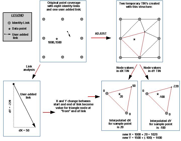
Rubbersheeting uses two temporary triangulated irregular networks (TINs) to interpolate changes in x (dX) and changes in y (dY) for feature coordinates along user-specified links. Each TIN has the same triangulation structure. The from-end of the displacement links and all identity links are used as the TIN triangle corners (nodes). A node is defined by its x,y location and a z value.
The z value of each node is used to interpolate the amount of x,y adjustment applied to each feature coordinate. The z value is the amount of change between the from-end and to-end of a link. For example, if the change in x for a link is 10 map units, the z value of the TIN node at the from-end of that link will be 10. Since identity links represent no change, the z value is zero. Once each node of a TIN triangle has a z value, the corresponding z value of any point falling on that triangle can be interpolated.
The interpolated z value from the x-shift TIN is added to the x ordinal of the feature's coordinate. The z value interpolated from the y-shift TIN is added to the y ordinal of the coordinate. For example, if an input feature coordinate is 1000,1500, the interpolated dX for this point is 20, and the interpolated dY is -100, the output coordinates after ADJUST will be 1020,1400 (1000 + 20 = 1020 and 1500 + (-100) = 1400).
The rubbersheeting adjustment has two options: linear and natural neighbor. These options refer to the interpolation method used to create the temporary TINs. You can read about these well-known mathematical models online or in the reference texts.
The linear method creates a quick TIN surface does not really take into account the neighborhood. It's quick and accurate if you have lots of displacement links over the area you are adjusting (that is, if the triangles are uniform).
Natural neighbor (similar to IDW) is slower but is more accurate when you don't have many displacement links and they are scattered across your dataset. Using linear in this case will be less accurate.
Edgematching
The edgematching process aligns features along the edge of one layer to features of an adjoining layer. It is mainly used when you want to merge separate adjacent layers such as soils or contours sheets etc and you need to ensure the features from those layers will meet at the join. The layer with the less accurate features is typically adjusted, while the adjoining layer is used as the control.

Attribute transfer
Attribute transfer is typically used to copy attributes from a less accurate layer to a more accurate one. For example, it can be used to transfer the names of hydrological features from a previously digitized and highly generalized 1:500,000 scale map to a more detailed 1:24,000 scale map. In ArcMap, you can specify what attributes to transfer between layers, then interactively choose the source and target features.
References
Maling, D.H. Coordinate Systems and Map Projections. George Philip, 1973.
Maling, D.H. "Coordinate Systems and Map Projections for GIS." In: Maguire, D.J., M.F. Goodchild, and D.W. Rhind (eds.), Geographical Information Systems: Principles and Applications. Vol. 1, pp. 135–146. Longman Group UK Ltd., 1991.
Moffitt, F.H., and E.M. Mikhail. Photogrammetry. Third Edition. Harper & Row, Inc., 1980.
Pettofrezzo, A.J. Matrices and Transformations. Dover Publications, Inc., 1966.
Slama, C.C., C. Theurer, and S.W. Henriksen (eds.). Manual of Photogrammetry. 4th Edition. Chapter XIV, pp. 729–731. ASPRS, 1980.
An overview of the spatial adjustment process
While each of the spatial adjustment functions are used for a different purpose, the steps for setting up and performing an adjustment are essentially the same.
- Start ArcMap.
Learn more about starting ArcMap
- Create a new map or open an existing one.
Learn more about creating a new map
- Add the data you want to edit to your map.
Learn more about adding data
- Add the Editor toolbar to ArcMap.
Learn more about adding the Editor toolbar
- Add the Spatial Adjustment toolbar to ArcMap.
Learn more about adding the Spatial Adjustment toolbar
- Start your edit session.
Learn more about starting an edit session
- Choose the input data for the adjustment.
Learn more about choosing input data for adjustment
- Choose a spatial adjustment method.
Learn more about choosing an adjustment method
- Create displacement links.
Learn more about creating displacement links
- Perform the adjustment.
Learn more about performing the adjustment
- Stop your edit session and save your edits.
There is no need to save the map—all edits made to the database will automatically be reflected the next time you open the map.
Learn more about opening a map
Learn more about stopping an edit session and saving your edits
Exploring the Spatial Adjustment toolbar
The Spatial Adjustment toolbar contains the various commands you will need to adjust geographic features in your map. You must add the Spatial Adjustment toolbar to ArcMap before you can begin adjusting data.
View the Spatial Adjustment toolbar