Show Navigation
|
Hide Navigation
How Hot Spot Analysis: Getis-Ord Gi* (Spatial Statistics) works |
|
|
Release 9.3
Last modified January 28, 2009 |


|
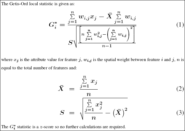
The Hot Spot Analysis tool calculates the Getis-Ord Gi* statistic for each feature in a dataset. The resultant Z score tells you where features with either high or low values cluster spatially. This tool works by looking at each feature within the context of neighboring features. A feature with a high value is interesting, but may not be a statistically significant hot spot. To be a statistically significant hot spot, a feature will have a high value and be surrounded by other features with high values as well. The local sum for a feature and its neighbors is compared proportionally to the sum of all features; when the local sum is much different than the expected local sum, and that difference is too large to be the result of random chance, a statistically significant Z score results.
Calculations

The p-values are numerical approximations of the area under the curve for a known distribution, limited by the test statistic. See What is a Z score What is a p-value.
Interpretation
The Gi* statistic returned for each feature in the dataset is a Z score. For statistically significant positive Z scores, the larger the Z score is, the more intense the clustering of high values (hot spot). For statistically significant negative Z scores, the smaller the Z score is, the more intense the clustering of low values (cold spot). See What is a Z score What is a p-value.Hot Spot Analysis
There are 3 things to consider when undertaking any hot spot analysis:- What is the Analysis Field? The hot spot analysis tool assesses whether high or low values (the number of crimes, accident severity, or dollars spent on sporting goods, for example) cluster spatially. The field containing those values is your Analysis Field. For point incident data, however, you may be more interested in assessing incident intensity than in analyzing the spatial clustering of any particular value associated with the incidents. In that case you will need to aggregate your incident data prior to analysis. There are several ways to do this:
- If you have census blocks or other polygon features for your study area, consider doing a Spatial Join to count the number of events in each block. The resultant field containing the number of events in each polygon becomes the Analysis Field.
- Use the Create Fishnet tool to construct a polygon grid over your point features. Then do a Spatial Join to count the number of events falling within each grid polygon. Remove any grid polygons that fall outside of your study area. Also, in cases where many of the grid polygons within the study area contain zeros for the number of events, increase the polygon grid size if appropriate, or remove those zero count grid polygons prior to analysis.
- Alternatively, if you have a number of coincident points or points within a short distance of one another, you can use Integrate with the Collect Events tool to (1) snap features within a specified distance of each other together and then (2) create a new feature class containing a point at each unique location with an associated count attribute to indicate the number of events/snapped points. Use the resultant ICOUNT field as your Analysis Field.
- Which Conceptualization of Spatial Relationships is appropriate? What Distance value is best? The recommended (and default) Conceptualization of Spatial Relationships for the Hot Spot Analysis tool is Fixed Distance. Zone of Indifference, Contiguity, K Nearest Neighbor and Delaunay Triangulation may also work well. For a discussion of best practices and strategies for determining an analysis distance value, see Selecting a Conceptualization of Spatial Relationships: Best Practices and also Selecting a Fixed Distance.
- What is the question? This may seem obvious, but how you construct the Analysis Field determines the types of questions you can ask. Are you most interested in determining where you have lots of incidents, or where high/low values for a particular attribute cluster spatially? If so, run Hot Spot Analysis on the raw values or raw incident counts. This type of analysis is particularly helpful for resource allocation types of problems. Alternatively (or in addition), you may be interested in locating areas with unexpectedly high values in relation to some other variable. If you are analyzing foreclosures, for example, you probably expect more foreclosures in locations with more homes (or said another way: at some level, you expect the number of foreclosures to be a function of the number of houses). If you divide the number of foreclosures by the number of homes, and then run the Hot Spot Analysis tool on this ratio, you are no longer asking "Where are there lots of foreclosures?"; instead you are asking "Where are there unexpectedly high numbers of foreclosures, given the number of homes?". By creating a rate or ratio prior to analysis, you can control for certain expected relationships (e.g., the number of crimes is a function of population; the number of foreclosures is a function of housing stock) and identify unexpected hot/cold spots.